Modernize fraud prevention: GraphStorm v0.5 for real-time inference

Fraud continues to cause significant financial damage globally, with U.S. consumers alone losing $12.5 billion in 2024—a 25% increase from the previous year according to the Federal Trade Commission. This surge stems not from more frequent attacks, but from fraudsters’ increasing sophistication. As fraudulent activities become more complex and interconnected, conventional machine learning approaches fall short by analyzing transactions in isolation, unable to capture the networks of coordinated activities that characterize modern fraud schemes.

Graph neural networks (GNNs) effectively address this challenge by modeling relationships between entities—such as users sharing devices, locations, or payment methods. By analyzing both network structures and entity attributes, GNNs are effective at identifying sophisticated fraud schemes where perpetrators mask individual suspicious activities but leave traces in their relationship networks. However, implementing GNN-based online fraud prevention in production environments presents unique challenges: achieving sub-second inference responses, scaling to billions of nodes and edges, and maintaining operational efficiency for model updates. In this post, we show you how to overcome these challenges using GraphStorm, particularly the new real-time inference capabilities of GraphStorm v0.5.

Previous solutions required tradeoffs between capability and simplicity. Our initial DGL approach provided comprehensive real-time capabilities but demanded intricate service orchestration—including manually updating endpoint configurations and payload formats after retraining with new hyperparameters. This approach also lacked model flexibility, requiring customization of GNN models and configurations when using architectures beyond relational graph convolutional networks (RGCN). Subsequent in-memory DGL implementations reduced complexity but encountered scalability limitations with enterprise data volumes. We built GraphStorm to bridge this gap, by introducing distributed training and high-level APIs that help simplify GNN development at enterprise scale.

In a recent blog post, we illustrated GraphStorm’s enterprise-scale GNN model training and offline inference capability and simplicity. While offline GNN fraud detection can identify fraudulent transactions after they occur—preventing financial loss requires stopping fraud before it happens. GraphStorm v0.5 makes this possible through native real-time inference support through Amazon SageMaker AI. GraphStorm v0.5 delivers two innovations: streamlined endpoint deployment that reduces weeks of custom engineering—coding SageMaker entry point files, packaging model artifacts, and calling SageMaker deployment APIs—to a single-command operation, and standardized payload specification that helps simplify client integration with real-time inference services. These capabilities enable sub-second node classification tasks like fraud prevention, empowering organizations to proactively counter fraud threat with scalable, operationally straightforward GNN solutions.

To showcase these capabilities, this post presents a fraud prevention solution. Through this solution, we show how a data scientist can transition a trained GNN model to production-ready inference endpoints with minimal operational overhead. If you’re interested in implementing GNN-based models for real-time fraud prevention or similar business cases, you can adapt the approaches presented here to create your own solutions.

Solution overview

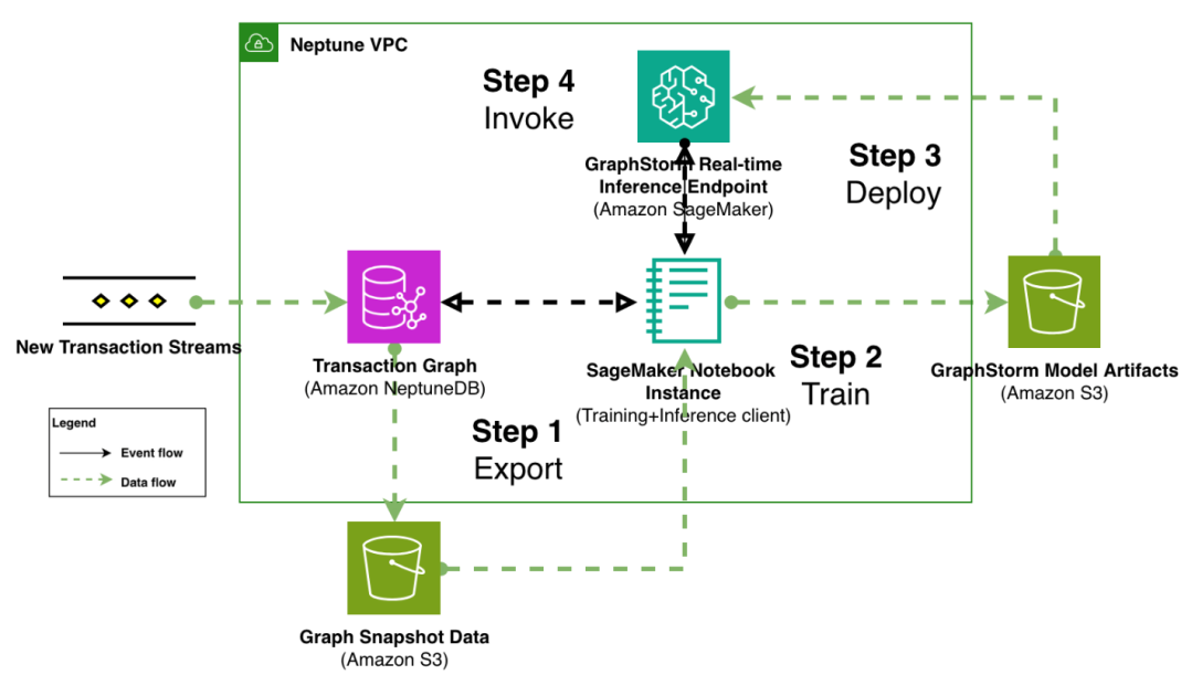
Our proposed solution is a 4-step pipeline as shown in the following figure. The pipeline starts at step 1 with transaction graph export from an online transaction processing (OLTP) graph database to scalable storage (Amazon Simple Storage Service (Amazon S3) or Amazon EFS), followed by distributed model training in step 2. Step 3 is GraphStorm v0.5’s simplified deployment process that creates SageMaker real-time inference endpoints with one command. After SageMaker AI has deployed the endpoint successfully, a client application integrates with the OLTP graph database that processes live transaction streams in step 4. By querying the graph database, the client prepares subgraphs around to-be predicted transactions, convert the subgraph into standardized payload format, and invoke deployed endpoint for real-time prediction.

To provide concrete implementation details for each step in the real-time inference solution, we demonstrate the complete workflow using the publicly available IEEE-CIS fraud detection task.

Note: This example uses a Jupyter notebook as the controller of the overall four-step pipeline for simplicity. For more production-ready design, see the architecture described in Build a GNN-based real-time fraud detection solution.

Prerequisites

To run this example, you need an AWS account that the example’s AWS Cloud Development Kit (AWS CDK) code uses to create required resources, including Amazon Virtual Private Cloud (Amazon VPC), an Amazon Neptune database, Amazon SageMaker AI, Amazon Elastic Container Registry (Amazon ECR), Amazon S3, and related roles and permission.

Note: These resources incur costs during execution (approximately $6 per hour with default settings). Monitor usage carefully and review pricing pages for these services before proceeding. Follow cleanup instructions at the end to avoid ongoing charges.

Hands-on example: Real-time fraud prevention with IEEE-CIS dataset

All implementation code for this example, including Jupyter notebooks and supporting Python scripts, is available in our public repository. The repository provides a complete end-to-end implementation that you can directly execute and adapt for your own fraud prevention use cases.

Dataset and task overview

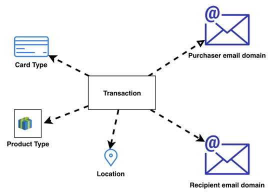
This example uses the IEEE-CIS fraud detection dataset, containing 500,000 anonymized transactions with approximately 3.5% fraudulent cases. The dataset includes 392 categorical and numerical features, with key attributes like card types, product types, addresses, and email domains forming the graph structure shown in the following figure. Each transaction (with an isFraud label) connects to Card Type, Location, Product Type, and Purchaser and Recipient email domain entities, creating a heterogeneous graph that enables GNN models to detect fraud patterns through entity relationships.

Unlike our previous post that demonstrated GraphStorm plus Amazon Neptune Analytics for offline analysis workflows, this example uses a Neptune database as the OLTP graph store, optimized for the quick subgraph extraction required during real-time inference. Following the graph design, the tabular IEEE-CIS data is converted to a set CSV files compatible with Neptune database format, allowing direct loading into both the Neptune database and GraphStorm’s GNN model training pipeline with a single set of files.

Step 0: Environment setup

Step 0 establishes the running environment required for the four-step fraud prevention pipeline. Complete setup instructions are available in the implementation repository.

To run the example solution, you need to deploy an AWS CloudFormation stack through the AWS CDK. This stack creates the Neptune DB instance, the VPC to place it in, and appropriate roles and security groups. It additionally creates a SageMaker AI notebook instance, from which you run the example notebooks that come with the repository.

git clone https://github.com/aws-samples/amazon-neptune-samples.git
cd neptune-database-graphstorm-online-inference/neptune-db-cdk
# Ensure you have CDK installed and have appropriate credentials set up
cdk deploy

When deployment is finished (it takes approximately 10 minutes for required resources to be ready), the AWS CDK prints a few outputs, one of which is the name of the SageMaker notebook instance you use to run through the notebooks:

# Example output
NeptuneInfraStack.NotebookInstanceName = arn:aws:sagemaker:us-east-1:012345678912:notebook-instance/NeptuneNotebook-9KgSB9XXXXXX

You can navigate to the SageMaker AI notebook UI, find the corresponding notebook instance, and select its Open Jupyterlab link to access the notebook.

Alternatively, you can use the AWS Command Line Interface (AWS CLI) to get a pre-signed URL to access the notebook. You will need to replace the with the actual notebook instance name.

aws sagemaker create-presigned-notebook-instance-url --notebook-instance-name 

When you’re in the notebook instance web console, open the first notebook, 0-Data-Preparation.ipynb, to start going through the example.

Step 1: Graph construction

In the Notebook 0-Data-Preparation, you transform the tabular IEEE-CIS dataset into the heterogeneous graph structure shown in the figure at the start of this section. The provided Jupyter Notebook extracts entities from transaction features, creating Card Type nodes from card1–card6 features, Purchaser and Recipient nodes from email domains, Product Type nodes from product codes, and Location nodes from geographic information. The transformation establishes relationships between transactions and these entities, generating graph data in Neptune import format for direct ingestion into the OLTP graph store. The create_neptune_db_data() function orchestrates this entity extraction and relationship creation process across all node types (which takes approximately 30 seconds).

GRAPH_NAME = "ieee-cis-fraud-detection"
PROCESSED_PREFIX = f"./{GRAPH_NAME}"
ID_COLS = "card1,card2,card3,card4,card5,card6,ProductCD,addr1,addr2,P_emaildomain,R_emaildomain"
CAT_COLS = "M1,M2,M3,M4,M5,M6,M7,M8,M9"
# Lists of columns to keep from each file
COLS_TO_KEEP = {
    "transaction.csv": (
        ID_COLS.split(",")
        + CAT_COLS.split(",")
        +
        # Numerical features without missing values
        [f"C{idx}" for idx in range(1, 15)]
        + ["TransactionID", "TransactionAmt", "TransactionDT", "isFraud"]
    ),
    "identity.csv": ["TransactionID", "DeviceType"],
}

create_neptune_db_data(
    data_prefix="./input-data/",
    output_prefix=PROCESSED_PREFIX,
    id_cols=ID_COLS,
    cat_cols=CAT_COLS,
    cols_to_keep=COLS_TO_KEEP,
    num_chunks=1,
)

This notebook also generates the JSON configuration file required by GraphStorm’s GConstruct command and executes the graph construction process. This GConstruct command transforms the Neptune-formatted data into a distributed binary graph format optimized for GraphStorm’s training pipeline, which partitions the heterogeneous graph structure across compute nodes to enable scalable model training on industry-scale graphs (measured in billions of nodes and edges). For the IEEE-CIS data, the GConstruct command takes 90 seconds to complete.

In the Notebook 1-Load-Data-Into-Neptune-DB, you load the CSV data into the Neptune database instance (takes approximately 9 minutes), which makes them available for online inference. During online inference, after selecting a transaction node, you query the Neptune database to get the graph neighborhood of the target node, retrieving the features of every node in the neighborhood and the subgraph structure around the target.

Step 2: Model training

After you have converted the data into the distributed binary graph format, it’s time to train a GNN model. GraphStorm provides command-line scripts to train a model without writing code. In the Notebook 2-Model-Training, you train a GNN model using GraphStorm’s node classification command with configuration managed through YAML files. The baseline configuration defines a two-layer RGCN model with 128-dimensional hidden layers, training for 4 epochs with a 0.001 learning rate and 1024 batch size, which takes approximately 100 seconds for 1 epoch of model training and evaluation in an ml.m5.4xlarge instance. To improve fraud detection accuracy, the notebook provides more advanced model configurations like the command below.

!python -m graphstorm.run.gs_node_classification \
           --workspace ./ \
           --part-config ieee_gs/ieee-cis.json \
           --num-trainers 1 \
           --cf ieee_nc.yaml \
           --eval-metric roc_auc \
           --save-model-path ./model-simple/ \
           --topk-model-to-save 1 \
           --imbalance-class-weights 0.1,1.0

Arguments in this command address the dataset’s label imbalance challenge where only 3.5% of transactions are fraudulent by using AUC-ROC as the evaluation metric and using class weights. The command also saves the best-performing model along with essential configuration files required for endpoint deployment. Advanced configurations can further enhance model performance through techniques like HGT encoders, multi-head attention, and class-weighted cross entropy loss function, though these optimizations increase computational requirements. GraphStorm enables these changes through run time arguments and YAML configurations, reducing the need for code modifications.

Step 3: Real-time endpoint deployment

In the Notebook 3-GraphStorm-Endpoint-Deployment, you deploy the real-time endpoint through GraphStorm v0.5’s straightforward launch script. The deployment requires three model artifacts generated during training: the saved model file that contains weights, the updated graph construction JSON file with feature transformation metadata, and the runtime-updated training configuration YAML file. These artifacts enable GraphStorm to recreate the exact training configurations and model for consistent inference behavior. Notably, the updated graph construction JSON and training configuration YAML file contains crucial configurations that are essential for restoring the trained model on the endpoint and processing incoming request payloads. It is crucial to use the updated JSON and YAML files for endpoint deployment.GraphStorm uses SageMaker AI bring your own container (BYOC) to deploy a consistent inference environment. You need to build and push the GraphStorm real-time Docker image to Amazon ECR using the provided shell scripts. This containerized approach provides consistent runtime environments compatible with the SageMaker AI managed infrastructure. The Docker image contains the necessary dependencies for GraphStorm’s real-time inference capabilities on the deployment environment.

To deploy the endpoint, you can use the GraphStorm-provided launch_realtime_endpoint.py script that helps you gather required artifacts and creates the necessary SageMaker AI resources to deploy an endpoint. The script accepts the Amazon ECR image URI, IAM role, model artifact paths, and S3 bucket configuration, automatically handling endpoint provisioning and configuration. By default, the script waits for endpoint deployment to be complete before exiting. When completed, it prints the name and AWS Region of the deployed endpoint for subsequent inference requests. You will need to replace the fields enclosed by <> with the actual values of your environment.

!python ~/graphstorm/sagemaker/launch/launch_realtime_endpoint.py \
        --image-uri .dkr.ecr..amazonaws.com/graphstorm:sagemaker-endpoint-cpu \
        --role arn:aws:iam:::role/ \
        --region  \
        --restore-model-path /models/epoch-1/ \
        --model-yaml-config-file /models/GRAPHSTORM_RUNTIME_UPDATED_TRAINING_CONFIG.yaml \
        --graph-json-config-file /models/data_transform_new.json \
        --infer-task-type node_classification \
        --upload-tarfile-s3 s3:// \
        --model-name ieee-fraud-detect

Step 4: Real-time inference

In the Notebook 4-Sample-Graph-and-Invoke-Endpoint, you build a basic client application that integrates with the deployed GraphStorm endpoint to perform real-time fraud prevention on incoming transactions. The inference process accepts transaction data through standardized JSON payloads, executes node classification predictions in a few hundreds of milliseconds, and returns fraud probability scores that enable immediate decision-making.

An end-to-end inference call for a node that already exists in the graph has three distinct stages:

1. Graph sampling from the Neptune database. For a given target node that already exists in the graph, retrieve its k-hop neighborhood with a fanout limit, that is, limiting the number of neighbors retrieved at each hop by a threshold.
2. Payload preparation for inference. Neptune returns graphs using GraphSON, a specialized JSON-like data format used to describe graph data. At this step, you need to convert the returned GraphSON to GraphStorm’s own JSON specification. This step is performed on the inference client, in this case a SageMaker notebook instance.
3. Model inference using a SageMaker endpoint. After the payload is prepared, you send an inference request to a SageMaker endpoint that has loaded a previously trained model snapshot. The endpoint receives the request, performs any feature transformations needed (such as converting categorical features to one-hot encoding), creates the binary graph representation in memory, and makes a prediction for the target node using the graph neighborhood and trained model weights. The response is encoded to JSON and sent back to the client.

An example response from the endpoint would look like:

{'status_code': 200,
 'request_uid': '877042dbc361fc33',
 'message': 'Request processed successfully.',
 'error': '',
 'data': {
    'results': [
            {
                'node_type': 'Transaction',
                'node_id': '2991260',
                'prediction': [0.995966911315918, 0.004033133387565613]
            }
        ]
    }
}

The data of interest for the single transaction you made a prediction for are in the prediction key and corresponding node_id. The prediction gives you the raw scores the model produces for class 0 (legitimate) and class 1 (fraudulent) at the corresponding 0 and 1 indexes of the predictions list. In this example, the model marks the transaction as most likely legitimate. You can find the full GraphStorm response specification in the GraphStorm documentation.

Complete implementation examples, including client code and payload specifications, are provided in the repository to guide integration with production systems.

Clean up

To stop accruing costs on your account, you need to delete the AWS resources that you created with the AWS CDK at the Environment Setup step.

You must first delete the SageMaker endpoint created during the Step 3 for cdk destroy to complete. See the Delete Endpoints and Resources for more options to delete an endpoint. When done, you can run the following from the repository’s root:

cd neptune-database-graphstorm-online-inference/neptune-db-cdk
cdk destroy

See the AWS CDK docs for more information about how to use cdk destroy, or see the CloudFormation docs for how to delete a stack from the console UI. By default, the cdk destroy command does not delete the model artifacts and processed graph data stored in the S3 bucket during the training and deployment process. You must remove them manually. See Deleting a general purpose bucket for information about how to empty and delete an S3 bucket the AWS CDK has created.

Conclusion

Graph neural networks address complex fraud prevention challenges by modeling relationships between entities that traditional machine learning approaches miss when analyzing transactions in isolation. GraphStorm v0.5 helps simplify deployment of GNN real-time inference with one command for endpoint creation that previously required coordination of multiple services and a standardized payload specification that helps simplify client integration with real-time inference services. Organizations can now deploy enterprise-scale fraud prevention endpoints through streamlined commands that reduce custom engineering from weeks to single-command operations.

To implement GNN-based fraud prevention with your own data:

• Review the GraphStorm documentation for model configuration options and deployment specifications.
• Adapt this IEEE-CIS example to your fraud prevention dataset by modifying the graph construction and feature engineering steps using the complete source code and tutorials available in our GitHub repository.
• Access step-by-step implementation guidance to build production-ready fraud prevention solutions with GraphStorm v0.5’s enhanced capabilities using your enterprise data.

About the authors

Jian Zhang is a Senior Applied Scientist who has been using machine learning techniques to help customers solve various problems, such as fraud detection, decoration image generation, and more. He has successfully developed graph-based machine learning, particularly graph neural network, solutions for customers in China, the US, and Singapore. As an enlightener of AWS graph capabilities, Zhang has given many public presentations about GraphStorm, the GNN, the Deep Graph Library (DGL), Amazon Neptune, and other AWS services.

Theodore Vasiloudis is a Senior Applied Scientist at AWS, where he works on distributed machine learning systems and algorithms. He led the development of GraphStorm Processing, the distributed graph processing library for GraphStorm and is a core developer for GraphStorm. He received his PhD in Computer Science from KTH Royal Institute of Technology, Stockholm, in 2019.

Xiang Song is a Senior Applied Scientist at AWS AI Research and Education (AIRE), where he develops deep learning frameworks including GraphStorm, DGL, and DGL-KE. He led the development of Amazon Neptune ML, a new capability of Neptune that uses graph neural networks for graphs stored in graph database. He is now leading the development of GraphStorm, an open source graph machine learning framework for enterprise use cases. He received his PhD in computer systems and architecture at the Fudan University, Shanghai, in 2014.

Florian Saupe is a Principal Technical Product Manager at AWS AI/ML research supporting science teams like the graph machine learning group, and ML Systems teams working on large scale distributed training, inference, and fault resilience. Before joining AWS, Florian lead technical product management for automated driving at Bosch, was a strategy consultant at McKinsey & Company, and worked as a control systems and robotics scientist—a field in which he holds a PhD.

Ozan Eken is a Product Manager at AWS, passionate about building cutting-edge Generative AI and Graph Analytics products. With a focus on simplifying complex data challenges, Ozan helps customers unlock deeper insights and accelerate innovation. Outside of work, he enjoys trying new foods, exploring different countries, and watching soccer.